- Creating Custom SQL Aggregations
- Creating Custom SQL Queries
- Custom SQL Aggregations - Examples
- Supported SQL Functions
Creating Custom SQL Aggregations
To create Custom SQL Aggregations in the m3ter Console you can follow similar steps as when you create other types of Aggregation using the standard aggregation methods, such as SUM, COUNT, MAXIMUM, and so on. To create a Custom SQL Aggregation:- Select Metering>Aggregations. The Aggregations page opens.
- In the Product drop-down, select the Product for which you want to create the new Custom SQL Aggregation.
- Select Create aggregation. The Aggregations>Create page opens.
- Configure Aggregation details and enter:
- Name. (Required)
- Code. (Required)
- Accounting product. Use the drop-down to select a Product. (Optional)
- For accounting purposes, you can use this to link to a specific Product any usage line items on Bills that result from pricing a Plan using this Aggregation:
- If you’ve also defined an Accounting product for a Pricing that uses this Aggregation, then the Pricing Accounting product takes precedence and is used.
- If no Accounting product is defined for a Pricing and you omit an Accounting product for the Aggregation, then the Product the Plan belongs to is used.
- For accounting purposes, you can use this to link to a specific Product any usage line items on Bills that result from pricing a Plan using this Aggregation:
- Configure Meter settings:
- Meter. Select the Meter whose Data Field or Derived Field you want to use as the basis for the Aggregation. Note that only those Meters created for the selected Product will be available. If you’re creating a Global Aggregation only Global Meters will be available.
- Target Field. When you select a Meter, the Target Field drop-down list automatically populates with the Codes of any fields set up on that Meter:
- Note that you must select a measure target field on the Meter - that is, of type Measure, Income, or Cost.
- Configure Aggregation settings:
- Aggregation. Select Custom SQL for the aggregation method. The page adjusts to show an SQL text entry box where you can enter your SQL query expression. For example:
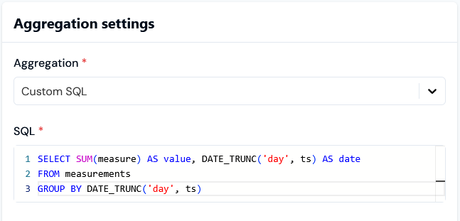
For details on creating Custom SQL queries for use in your Aggregations, please see the following Creating Custom SQL Queries section.
- Unit. This will be used as a label for billing to indicate to your customers what they are being charged for.
- Quantity per unit. Enter the quantity by which you want to charge for the measured value.
- Rounding. Specifies how you want m3ter to deal with non-integer, that is fractional number, Aggregation values.
- Select Create aggregation. The Aggregation details page opens:
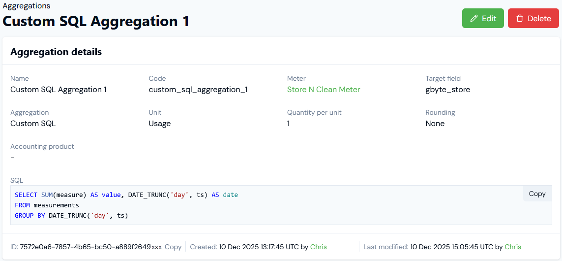
- Read-off the Aggregation’s Name and Code.
- Use a hotlink text to open the details page of the Meter whose Data Field the Aggregation targets.
- Review the SQL and Copy this to your clipboard.
- Note that for this example, because the selected Meter Target field for the Aggregation is
gbyte_store, then it is this field that is accessible in SQL as a field calledmeasure.
- Note that for this example, because the selected Meter Target field for the Aggregation is
- Check the Unit configured for the Aggregation, which will be used on Bill line items to indicates what the charge is for.
- Copy the Aggregation’s ID to your clipboard.
- Check the audit data to see who Created and who Last modified the Aggregation.
Creating Custom SQL Queries
This section provides details and guidance for creating queries for your Custom SQL Aggregations. Please review this section in preparation for creating Custom SQL queries:Measurements Table
Custom SQL queries should be run against the measurements table. This table is provided to your SQL query and is already limited to the appropriate Account, time period, and so on that the Aggregation needs to run over, so you don’t need to include anything in your own SQL for these factors. Several columns of themeasurements table are made available to your Custom SQL queries:
| Column | Type | Used for |
|---|---|---|
| measure | Float64 | The value of the target field you selected. |
| ts | DateTime64 | The ts value of the measurement in UTC timezone. |
| ets | DateTime64 | The ets value of the measurement in UTC timezone. |
| uid | String | The uid value of the measurement. |
| received_at | DateTime64 | When the data was received in UTC timezone. |
| account_id | UUID | |
| dimensions | Map of Strings | String dimension values for the measurement. |
Key Points
When creating your SQL queries, please note the following key points:- The result(s) of the query must be returned as a numeric column called value.
- Queries can return up to 1,000 rows.
- Any additional columns returned (apart from value) are treated as “group keys” and are used downstream – this can be useful if the query returns multiple rows to help identify each row.
- If there are multiple rows, each row will be rated independently and appear as separate line items on the Bill.
- Dimensions can be accessed using map notation. For example, to access the value of a dimension called “region”, you would write
dimensions['region']. - The group key values can be accessed in line item descriptions using the syntax
{group.columnName}(wherecolumnNameis the name of the column you returned from your custom SQL query).
Limit on GROUP BY Clause
The limit on the use of GROUP BY clauses for a Custom SQL Aggregation depends on whether or not the Aggregation is segmented. This is because the “unique keys” in the operation will implicitly include segments:- An SQL query on an unsegmented Aggregation could process up to 50,000 unique keys from custom SQL.
- An SQL query on a segmented Aggregation will use some of those keys for the segment values (up to 1,000 depending on the data). In the worst case, if the data actually contained 1,000 different segment values, you’d only have 50 unique values for your own data that you are grouping by. This is because each of your own “keys” would be multiplied by (up to) 1,000 segment values,
- For example, if your data had keys of “a”, “b”, and “c”:
- An unsegmented Aggregation would see these 3 keys.
- However, if you segmented the Aggregation and each of your groups contained data for 3 segments: “1”, “2”, and “3”, then the total number of keys “seen” by the query will be:
- “a”, “1”
- “a”, “2”
- “a”, “3”
- “b”, “1”
- “b”, “2”
- “b”, “3”
- “c”, “1”
- “c”, “2”
- “c”, “3”
Custom SQL Aggregations - Examples
This section offers some example billing use cases fulfilled using Custom SQL Aggregations:- Example 1 - Monthly Billing, Daily Rating
- Example 2 - Group by Dimension
- Example 3 - Reserved Instances (RIs) with Overages
- Example 4 - Custom SQL Descriptions
Example 1 - Monthly Billing, Daily Rating
In this example you have tiered pricing with a usage allowance that resets daily - but you bill monthly. This use case is simple to fulfill with Custom SQL Aggregations - we can group by the day based on the measurement timestamp:Example 2 - Group by Dimension
Suppose you price based on a simple total of the distance driven by vehicles each month. Each measurement has a dimension ofvehicle_id on it, indicating which vehicle drove a certain distance.
Currently, we support taking a SUM over the entire dataset, regardless of the value of the vehicle_id field. We also support segmentation, but to configure segments you’d need to know and configure the vehicle ids ahead of time, and there’s a per-Organization limit of 1000.
This means that before Custom SQL Aggregations, for non-trivial pricing (such as tiered or volume pricing) the final cost is determined by the total distance driven by all vehicles combined.
Instead, we want to rate each vehicle independently, so that the first 100 miles driven by each vehicle is more expensive than subsequent miles. This would be possible by writing custom SQL which groups the total distance traveled by vehicle_id as follows:
distance(a measure field)vehicle_id(a dimension field)
distance as the target field in the Custom SQL Aggregation configuration, which is then accessible in SQL as a field called measure.
Example 3 - Reserved Instances (RIs) with Overages
You can reference Counter values from Custom SQL using the syntax:- The Reserved Instance (RI) rate is $2.50 per CPU per month.
- The overage on-demand (OD) rate is $0.005 per CPU-hour, which is more expensive per month than the RI rate, at roughly £3.60 for a 30-day month.
- Usage is monitored, and every hour one measurement is sent to m3ter indicating how many CPUs the end-customer actually using during that hour.
- By around mid-month, the end-customer realizes they are using more compute resource than expected, so they increase their number of Reserved Instances to 20 on the 15th of the month.
ri for the number of Reserved Instances, which is initially set to 10 and increased to 20 on the 15th. The Counter pricing for the RIs is set to $2.50, that is, the cost of 1 RI per month.
The Bill for the month is calculated and we get the usual Counter line items, giving us a line item of $38.71 for the RIs:
- Assuming a 31-day month and because the end-customer increased their RIs from 10 to 20 on the 15th of the month, the costs due under the Counter pricing we’ve set up is pro-rated for the Bill calculation:
- (14/31)*10(CPUs) + (17/31)*20(CPUs) = 15.4838709677 CPUs, which at a rate of $2.50 per CPU per month costs $38.71.
- 1st-14th : $25.20 (14*24*15*0.005$)
- 15th-31st: $10.20 (17*24*5*0.005)
- The total bill covering both Reserved Instances and on-demand overages is therefore: $38.71 + $25.20 + $10.20 = $74.11.
Example 4 - Custom SQL Descriptions
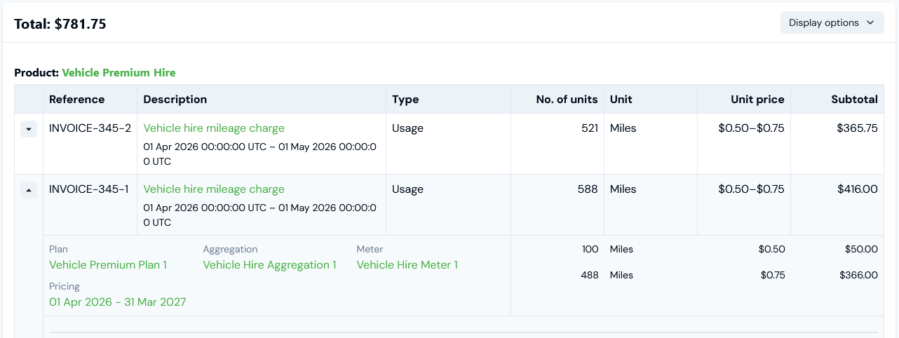
If you are using Custom SQL Aggregations to price Plans, this feature offers you wide flexibility when setting up Bill line item descriptions. Suppose you run a vehicle hire business and want to charge your customers for vehicle hire usage and invoice them monthly for vehicle distances recorded on a per-car basis. To do this, we can set up a Meter as follows: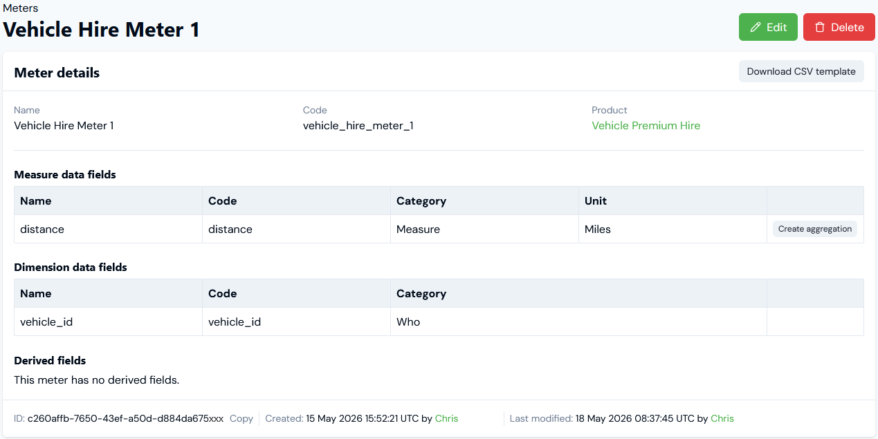
distance Meter’s Measure Data Field and groups by the vehicle_id Dimension Data Field:
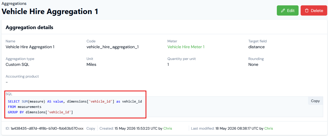
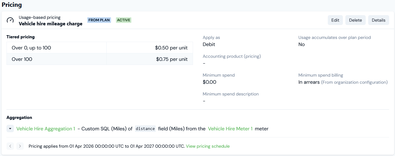
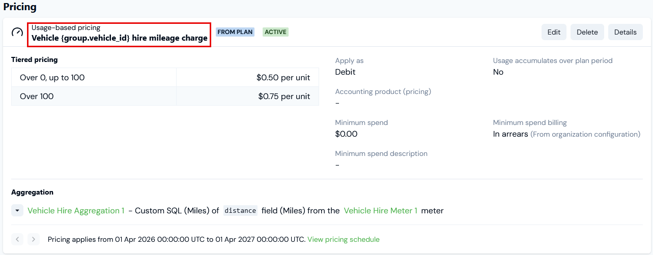
- Use Vehicle Hire Aggregation 1 to price a Plan we’ve attached to the customer Account:
- Define a two-tiered pricing.
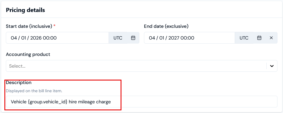
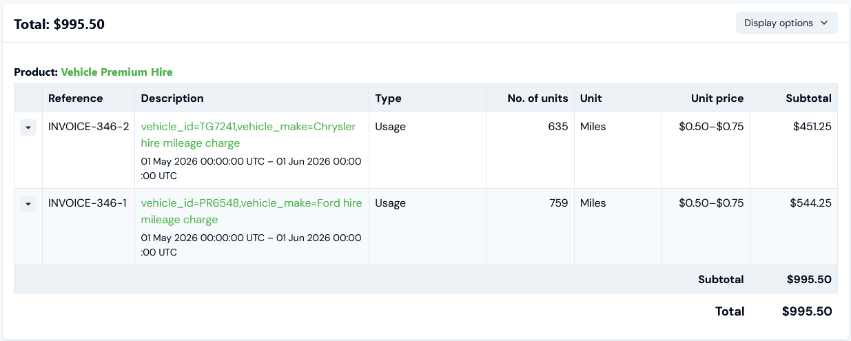
- Define a generic description: Vehicle hire mileage charge.
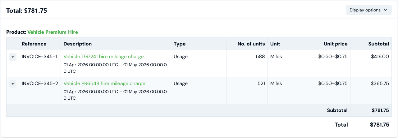
- If we make some test usage data submissions for a customer Account using Vehicle Hire Meter 1 for the month of April 2026 and for two vehicles, we can check the submissions in Usage Data Explorer:
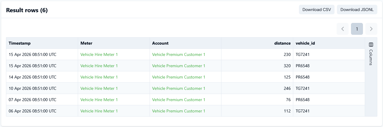
vehicle_id dimension used in the Custom SQL to GROUP BY:
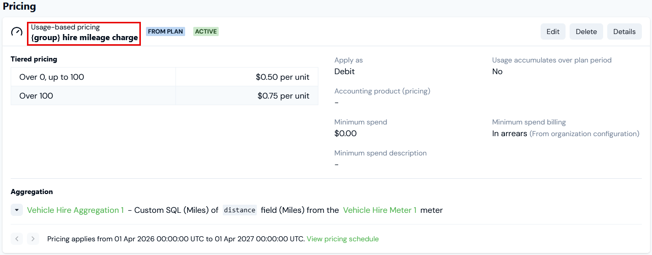
- Add a
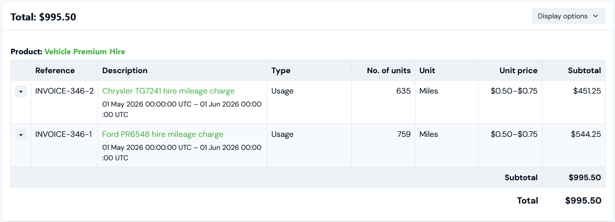
vehicle_makedimension Data Field to the Meter. - Adjust the Aggregation’s SQL to GROUP BY this second dimension:

vehicle_make Meter Data Field and continue to use the same pricing description for group:


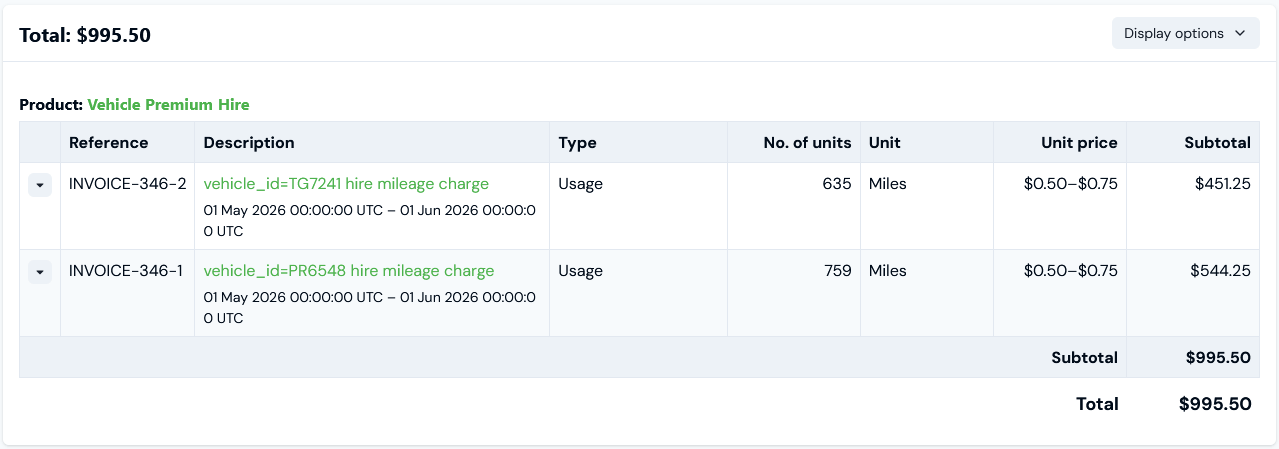
Default Custom SQL Descriptions
If you do not define a description on the pricing you configure for a Plan using a Custom SQL Aggregation, then a default description is used that includes any key/value pairs used in the GROUP BY clause: <Aggregation name> (<key/value 1>,<key/value 2>, <key/value 3>…) For the current example, the default description format resolves to: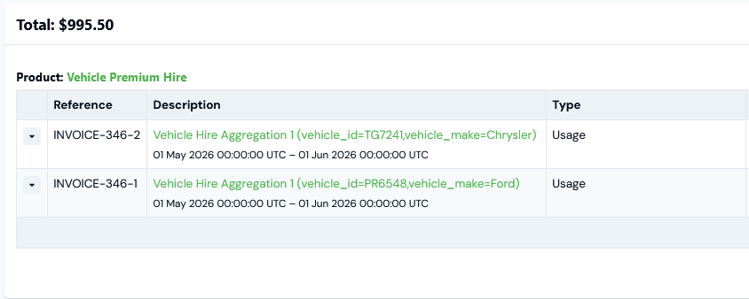
Supported SQL Functions
The following functions are supported in Custom SQL Aggregations:AVGCASTCEILCOALESCECOUNTDATE_TRUNCFIRST_VALUEFLOORGREATESTLAST_VALUELEASTMAXMINORDER_BYROUNDROW_NUMBERSUM